test
Click n click (GC606J1)

Today’s puzzle is a single part of a mystery that comprises several smaller puzzles, styled on the cult classic TV show The Crystal Maze. To get the coordinates there is a “mental” test for the northings, two easy puzzles that I won’t go into here. The westings are the more interesting part, with a “skill” test.
The skill test is a whack-a-mole game, with 60 radio buttons. One radio button is highlighted at random and you need to click it. If you hit, you get a point, and if you miss, you lose a point. After 30 seconds, if your score is 30 or more, you are presented with the coordinates. Now, there’s more than one way to skin this particular cat, and one of them doesn’t require any fast fingers or making an R programme. But I’ll stay silent on that method and instead use the opportunity to demonstrate how sometimes R can be enhanced by invoking scripts in other languages.
R seems to lack a way to read information about pixels on the screen. It’s easy to do if you’re interested in pixels within an image, but in this case we’re not. I’d like to read the pixels on the screen to detect which radio button is lit, then direct the mouse to click there. So I cribbed a small python script from somewhere or other to plug the gap of detecting the colour:
def get_pixel_colour(i_x, i_y):
    import win32gui
    i_desktop_window_id = win32gui.GetDesktopWindow()
    i_desktop_window_dc = win32gui.GetWindowDC(i_desktop_window_id)
    long_colour = win32gui.GetPixel(i_desktop_window_dc, i_x, i_y)
    i_colour = int(long_colour)
    return (i_colour & 0xff), ((i_colour >> 8) & 0xff), ((i_colour >> 16) & 0xff)
The reticulate package allows us to take a python function and “source” it, loading it as though it is an R function. It’s really painless. KeyboardSimulator can send key presses and mouse clicks to the OS. And those two packages do most of the hard work. Here’s the code:
library(KeyboardSimulator)
library(reticulate)
library(magrittr)

## the source_python takes a few seconds to run, and we're against the clock in this game
## so the first run will stop after it's in memory, and the second run will ignore this block
if (exists("runBefore")==0) {
  runBefore <- 1
  source_python("C:/Users/alunh/OneDrive/Documents/Repos/geo2/getPixelColour.py")
  stop("python script loaded!")
}

## the position of the radio buttons on my screen
w <- 26
h <- 21
l <- 1324
t <- 290

## the target radio button is dark grey and the non-targets are pale.
## Choose r+g+b < 500 to identify the target
start <- Sys.time()
repeat {
  for (x in sample(10)) {
    for (y in sample(6)) {
      ## here's the python function!
      p <- get_pixel_colour(as.integer(l+w*(x-1)), as.integer(t+h*(y-1))) %>%
        unlist()
      if (sum(p) < 500) {
        mouse.move(l + w * (x-1), t+h * (y-1))
        mouse.click()
      }
    }
  }
  ## quit after 32 seconds
  if ((Sys.time() - start) > 32) break
}
So how did our R/python hybrid do? Remember, the target was 30 correct clicks within 30 seconds, without errors. Using a mouse, I managed 23, and using a touchscreen device I made it to 34.

51! Not too shabby! Doubtless something bigger and better could be done to improve this score, but I’m very satisfied with my first foray into sourcing python from R.
It’s not often that R has a gap in its functionality, and there might well be a way of doing this without resorting to a python script. Please let me know if you have a better way by using the comment section below.
Plotting Pairs (GC4W6HJ)

Planning for a trip to Cornwall, I was churning through some mysteries there, largely picking them at random from the map. I worked my way through this one by hand, copying the puzzle into a text editor and separating the pairs manually before finally transferring it into RStudio and plotting the result. I moved on.
Later, I twigged that this would be an ideal demonstration of several powerful aspects of string manipulation in R, so I returned and wrote a program to do the same.
The puzzle is straightforward: just plot the coordinate pairs and you should see the cache coordinates spelled out in your plot.
I chose to use a regular expression to extract the contents of each pair of parentheses, using the str_extract_all function from the stringr package. This “regex” approach is powerful but also makes for a daunting read. If you are new to regular expressions, this website can help you understand them a little better. There is also a cheatsheet section to help remind more experienced users. Regular expressions are definitely worth the trouble.
library(tidyverse)
library(magrittr)
library(stringr)
B10 <- "(-3,-1)(-3,-5)(-2,-3)(-1,-5)(-1,-1) (-8,9)(-10,9)(-10,7)(-9,7)(-8,5)(-10,5) (-7,5)(-7,9)(-5,9)(-5,5)(-7,5) (-5,-6)(-6,-8)(-6,-10)(-4,-10)(-4,-8)(-6,-8) (2,9)(1,7)(1,5)(3,5)(3,7)(1,7) (5,-8)(3,-8)(3,-10)(5,-10)(5,-6)(4,-6)(4,-8) (2,-1)(0,-1)(0,-3)(1,-3)(2,-5)(0,-5) (2,-6)(0,-6)(0,-8)(1,-8)(2,-10)(0,-10) (-13,5)(-13,9)(-11,5)(-11,9) (12,7)(10,7)(10,5)(12,5)(12,9)(11,9)(11,7) (-1,-8)(-3,-8)(-3,-6)(-1,-6)(-1,-8)(-2,-10) (8,9)(7,7)(7,5)(9,5)(9,7)(7,7) (4,5)(4,9)(6,9)(6,5)(4,5) (-2,8)(-1,9)(-1,5)"

B10 %>%
  str_extract_all("(?<=\\()([^\\(\\)]+)(?=\\))") %>%
  unlist() %>%
  paste(collapse=",") %>%
  str_split(",") %>%
  unlist() %>%
  as.numeric() %>%
  matrix(ncol = 2, byrow = TRUE) %>%
  plot(type="l")
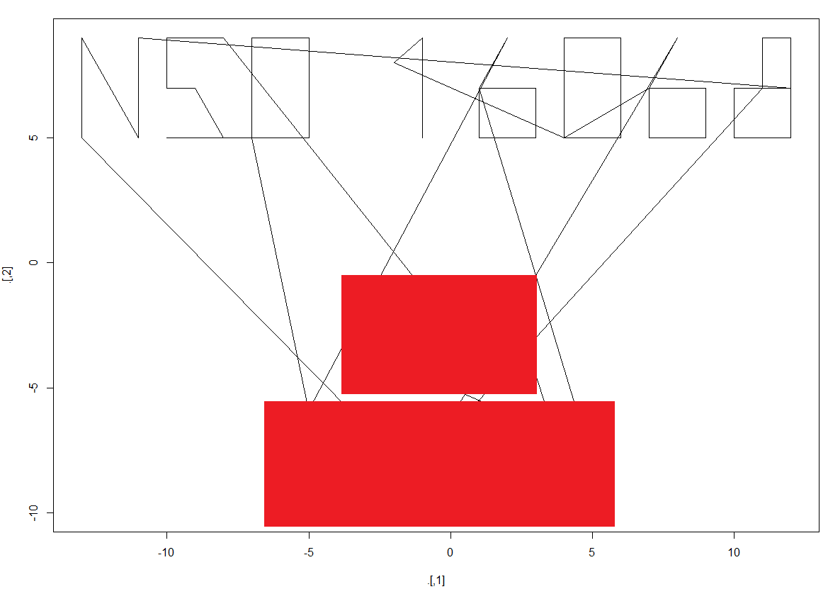
I chose to collapse the pairs of numbers into one big vector and make them into a matrix, which I then plotted with a line plot. It’s not tidy because of the lines joining different characters, but it’s legible.
I just noticed that there are spaces in the original text, probably to separate individual characters. Therefore I could have made something even more sophisticated, separating by spaces first and producing a tidier plot. But I’ve solved this puzzle twice now; a third time just for perfection would be overkill.
The bulk of the work in this puzzle is preparing the data, which is similar to many data visualisation or analysis workflows. stringr is the main engine of my solution, plucking the pairs from the parentheses, and again splitting them by the separator in order to coerce messy character data into a clean set of numbers that can be plotted. And it’s scalable, unlike the by-hand method I first used. This task involved 156 numbers, but it could just as easily have been 1560, making the manual approach a poor use of solving time.
GC4XMN7 RR138 – 404 Found

It’s been a few weeks since I found a puzzle worth programming in R, so I turned back to the RR series in the east of England to see if there was another, and there is.
The cache page shows a quite unilluminating image, mostly white with a couple of small characters. Opening the image in a new tab, I could see the image was similar but different. Ok, so this is one of those caches where PHP is used to serve up an image that changes. Sometimes these can be tricky, involving long waits, or lots of gathering information before you can even see the extent of the puzzle. But I suspected this one was more straightforward: it would be just a case of gathering a bunch of the images and overlaying them on each other to show the letters all in single frame. I shudder to think how I would go about this without R, so let’s get coding:
library(caTools)
library(abind)
library(magrittr)
URL <- "http://infin.ity.me.uk/MyCaches/RR138/RR138.php"
dr <- "C:/Users/alunh/OneDrive/Documents/Repos/geo2/Solving/GC4XMN7_rr138-404-found/"
for (q in 1:80) {
  tid <- as.character(round(as.numeric(Sys.time())*1000, 0))
  download.file(URL, destfile = paste0(dr, tid, ".gif"), mode = 'wb')
} # download 80 versions of the image
lapply(
  list.files(dr, full.names = TRUE, pattern="gif"),
  function(q) {
  read.gif(filename = q)$image
}
) %>%
  c(list(along=3)) %>%
  do.call(what=abind) %>%
  apply(1:2, max) %>% # every time a non-black pixel is found, preserve it
  apply(1, rev) %>% # this is a lazy way of rotating the matrix so it image()s the right way up
  apply(1, rev) %>% # this is a lazy way of rotating the matrix so it image()s the right way up
  apply(1, rev) %>% # this is a lazy way of rotating the matrix so it image()s the right way up
  image(col=c("black", "white"))
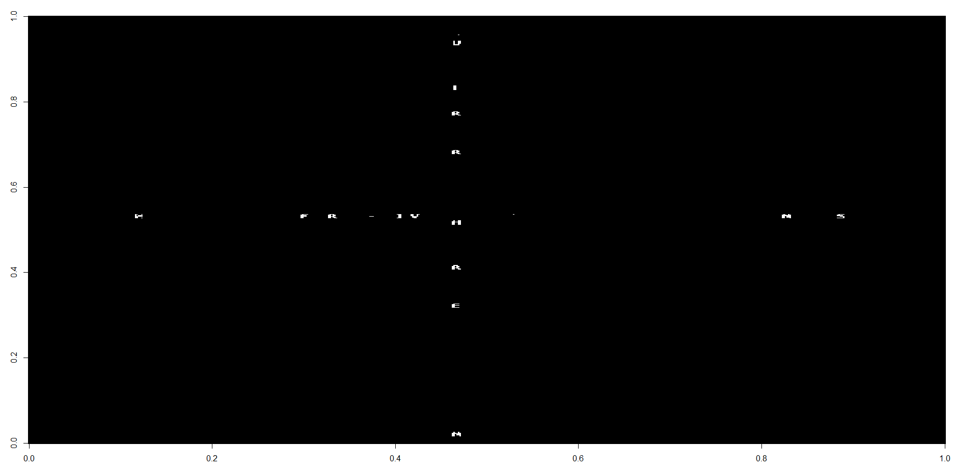
The image shows the partial result of the plot (I’ve kept it partial to avoid spoilers), but the pattern is clear: a cross of letters, spelling out the north coordinates vertically and the east coordinates horizontally. Job done!
It took a little searching to remind myself how to read in GIFs — the caTools library is the answer. It’s a slight oddity that there isn’t a package called gif, analogous to the jpeg and png packages, but there’s no gap in the functionality.
Also putting in a welcome appearance is one of my favourite R tricks, rotating a matrix using the simplest of commands: apply(m, 1, rev). I don’t mind admitting I get a frisson of pleasure whenever I get to use that, because it’s so elegant.
Last time, I mentioned that I “discovered” a new integer sequence. After a length submission and review process, it was found that I hadn’t, in fact. I’d just found an existing one and put a slightly odd twist on it. I withdrew my submission, but my thanks go to the editors of oeis.org for their patience and diligence in dealing with my attempt to get my name into that most nerdy hall of fame. One day.
GC5GRBF RR175 – Polymath

There is a series of puzzle caches in the east of England with a great number of interesting abstract puzzles, some of which are R-able. Amongst this estimable collection is one which is itself a miniature collection of puzzles. I saw it yesterday and starting working on the fifteen small puzzles. As of writing this, I’ve finished 10 of them and, to congratulate myself, I’m taking time off to share one of them, since it’s lead to something of a discovery. First the puzzle:
The number 720 has no fewer than 29 divisors: 1, 2, 3, 4, 5, 6, 8, 9, 10, 12, 15, 16, 18, 20, 24, 30, 36, 40, 45, 48, 60, 72, 80, 90, 120, 144, 180, 240 and 360. But 29 is not the “record”. Another three-digit number exists which has 31 divisors? Can you find it?
A heuristic method occurred to me: a way to produce a minimal product with maximal divisors, which popped into my head and took me quickly to a possible solution. The method then slipped into haze and I can no longer describe it well*, but even if it was sound, and I can’t be sure, it’s safest to check my answer methodically. Here’s a quick R programme to do that
library(tidyverse)library(magrittr)## a function to find the integer partitions of a given numberdivisors <- function(x) {if (x < 4) return(1)tries <- 2:sqrt(x)exact <- (x / tries) %% 1c(1, tries[exact==0], x/tries[exact==0]) %>% unique() %>% sort()}## vectorising inputs to a given maximumdivisor_progress <- function(n) {sapply(1:n, function(q) {q %>% divisors() %>% length()}) %>% cbind(x=1:n, y=.)}## show the answerdivisor_progress(999) %>% as_tibble() %>% arrange(-y)
The answer I came up with was quickly confirmed. But I didn’t stop to go back to the other puzzlettes; I started to explore the pattern of the increasing number of divisors in the sequence of positive integers.
There is an incredible resource online called the Online Encyclopedia of Integer Sequences which you can see here. Beware, for a number nerd it is pure quicksand. I’ve seldom found a website that I could spend so long just browsing, and I really thought that they had everything in there that I could ever hope to come across. Wrong. The number sequence I discovered was not in there. A close cousin is, but not mine. I did the responsible thing and signed up for an account and submitted it. I’ll update this blog when I hear back about its acceptance or rejection.
* but I’ll try
Write down a grid of prime numbers and increasing exponents to their right (I’ve kept them all below 100 just to make it tidy):2 4 8 16 32 643 9 27 815 257 491113
Then, take the smallest number you can find and include its base in your product. So first up we take the 2 in the top row. Its base is 2, so our first term is simply 2. Now, take the lowest unused element from the table. That’s the 3 in the second line. Our product is now 2*3 = 6. Next is the 4 from the first line, whose base is 2 again. 2*3*2 = 12. Eventually we get to 2*3*2*5*7*2, which is our answer.
This method, which is the result of a flash of insight rather than a rigorous analysis, might be wholly flawed, but it did get me to the right answer in this case, and the intermediate steps (6, 12, 60, 420) each seem to be standout local maxima for their number of divisors. If anyone has any insight into why this works, or why it is flawed, is encouraged to let me know!
GCTV41 Magic Eye View
Remember Magic Eye pictures? It was a craze in the 1990s where you would get books of abstract Pollockesque images, and, using a special technique, you could see a “3D” image. The technique, which I could never properly master, was to see “through” the page, focusing your gaze on a point behind the paper. The images are constructed in a such a way that that a subtly repeating pattern in the splodges tricked your brain into seeing the flat swirls of colour as contoured, and shapes would loom out of the paper.
I never quite mastered it, in the sense that I could only do it by crossing my eyes, meaning I was focusing in front of the page. It was effective in a sense: I could see three dimensional images, but they were recessed into the page instead of leaping off the page towards me.

This puzzle has its coordinates hidden in a magic eye picture. And I thought: what about those who’ve never mastered the art of magicking the hidden shapes off the page? I’m sure that’s something we can achieve with R, right?
The key to this is understanding that the image is largely a repeating horizontal pattern. The subtle differences are what gives us the 3D effect, but underpinning it is a regular pattern that we can exploit. If we can overlay two versions of the same image, offset horizontally by just the right amount, the difference between them should give us an image of the hidden shapes.
I could have sought to automatically detect the optimum distance — and that would still make a fascinating task some day — but I chose what felt to me the easier option. I built a Shiny package with a simple slider where the user specifies the offset, in pixels. Beneath that, an image dynamically shows the difference between images.
I had to consult the help files for renderImage and I was a bit worried that the process might be a bit clunky, since the jpg matrix is saved as a file which is then reloaded into the app. That read-write overhead seemed like a potential bottleneck, but when I ran it it responded well. Furthermore, the temporary file it creates each time the slider is adjusted is deleted straight after rendering, meaning I didn’t create digital clutter.
Here’s the start state of the app. The image is totally black because the two copies are aligned, and there is no difference.:

As I shift the slider along, I watch the patterns rising and falling…

Here’s the full code:
library(shiny)
library(jpeg)
library(abind)
magic <- readJPEG("c:/Users/alunh/OneDrive/Documents/Repos/geo2/Solving/GCTV41_magic-eye-view.jpg")
ui <- fluidPage(
sliderInput(inputId = "offset", label = "Offset in pixels", min = 0, max = 200, value = 0, step = 1),
imageOutput(outputId = "imag", height = "300px")
)
server <- function(input, output, session) {
output$imag <- renderImage({offset <- input$offsetmagic1 <- magic %>% abind(array(0, replace(dim(magic), 2, offset)), along = 2)
magic2 <- magic %>% abind(array(0, replace(dim(magic), 2, offset)), ., along = 2)
magicdiff <- magic1 - magic2
outfile <- tempfile(fileext='.jpg')
writeJPEG(magicdiff, outfile)
list(src=outfile, alt="..magic!")
})
}
shinyApp(ui, server)
Yeah, that’s pretty minimal for something so powerfully interactive. Shiny is not without its flaws, but it does the heavy lifting for you if you want a quick interactive app, and it’s a major selling point for the R programming language.
Here’s the final image, where you can just see the N51 and W002 start of the final coordinates. I hidden the full solution out of respect to the cache owner.

GC7X6EW MIND-BENDER

I stumbled upon a nice little puzzle in Gloucestershire, England:
Arrange the numbers 1 to 16, so each two numbers next to each other, add up to a square number. (You can only use each number once).
Devastatingly succinct. But potentially tricky. I reached out, as I always do, to R to help narrow the possibilities:
library(tidyverse)
library(magrittr)v <- 1:16
dafr <- crossing(a=v, b=v) %>%
filter(a < b) %>%
mutate(s = a + b) %>%
filter((a + b) %in% ((1:5)^2)) %>%
print()
Here made every combination of two different numbers, summed each pair and thrown out all the ones that don’t sum up to 1, 4, 9, 16, or 25. And there are only sixteen pairs remaining! We need fifteen, and each number must be used at most twice. Two numbers appear three times, so that is the rogue pair which can be discarded.
Furthermore, two numbers can only form a square-pair once each: 8 (which when added to 1 makes 9), and 16 (which makes 25 in combination with 9). They become our end members:
8 ... 16
And since their partners are known,
8 1 ... 9 16
Now it’s a purely mechanical task of picking out the remaining pair for each number, working towards the middle. Try it!
GC7J2FG Thorney Ramble – a QuarteR way down
Today’s puzzle takes us to the south of England, and it looks to me like an obfuscated QR code. Not only is this hinted at in the title, with Q and R in upper case, but the binary starts with a string of seven 1s. That’s a great heuristic for spotting this kind of QR-obfuscation.
I’m using RStudio, so displaying an image on the screen is a doddle:
library(magrittr)library(stringr)"1111111001001010101111111 1000001000111100001000001 1011101011101100101011101 1011101001110101101011101 1011101000100101101011101 1000001001000100001000001 1111111010101010101111111 0000000011101011100000000 1110111110111000111000100 1010010000110111001101011 1101111011001010100010101 0001000110010101000010011 0101111110010010011110000 0101010011001101111101100 1011111100001010101101111 0110100010010101010110001 1001111011011010111111011 0000000011011101100011010 1111111010010111101011011 1000001011010101100011000 1011101010010000111110011 1011101000011101001111010 1011101010010011111110101 1000001011010010001110010 1111111011011000010101111" %>%str_replace_all(" ", "") %>%strsplit("") %>%unlist() %>%as.numeric() %>%matrix(., ncol=sqrt(length(.))) %>%image(axes=FALSE, col=c("#ffffff", "#000000"))
That prints an output to the Plots window in RStudio:

Scanning the QR code with my phone reveals the coordinates; easy peasy!
GC4F5HY Shredded – JPS09
This puzzle is in Jersey and features an image, which, judging by the colours and rough shape, is obviously a scrambled version of a map of Jersey. The text confirms that a map has been “shredded”, and your task is to unshred it.

I’m intrigued to know how they did this in the first place — I sincerely hope it wasn’t done by hand. There are 100 slices there, and it’d take forever to do using Photoshop. Similarly, I didn’t want to stitch it back together by hand, so… what about the programmatic approach?
There are two main challenges here. Firstly, I need to divide the image up correctly. Luckily, the cache owner has left a couple of pixels’ white space between each strip. That should be easy to detect. Secondly, we have to decide how to stick them back together. The way I chose to do this was to take the right-hand edge of one strip, and compare the RGB values from the left hand edges of the others. Whichever one gives the best match gets glued on, and we start again, repeating until we have just one strip left.
I’m using the jpeg package, which converts a jpeg file into a three dimensional array representing the red, green and blue pixels.
library(jpeg) library(plyr) library(tidyverse) library(magrittr) library(abind)## get the imagedr <- "C:/Users/alunh/OneDrive/Documents/Repos/geo2/Solving/" shred <- readJPEG(paste0(dr, "GC4F5HY_shredded-jps09.jpg")) * 255## find the white lineswhiteness <- apply(shred, 1:2, sum)strips <- whiteness %>% apply(2, sum) strips %>% plot()
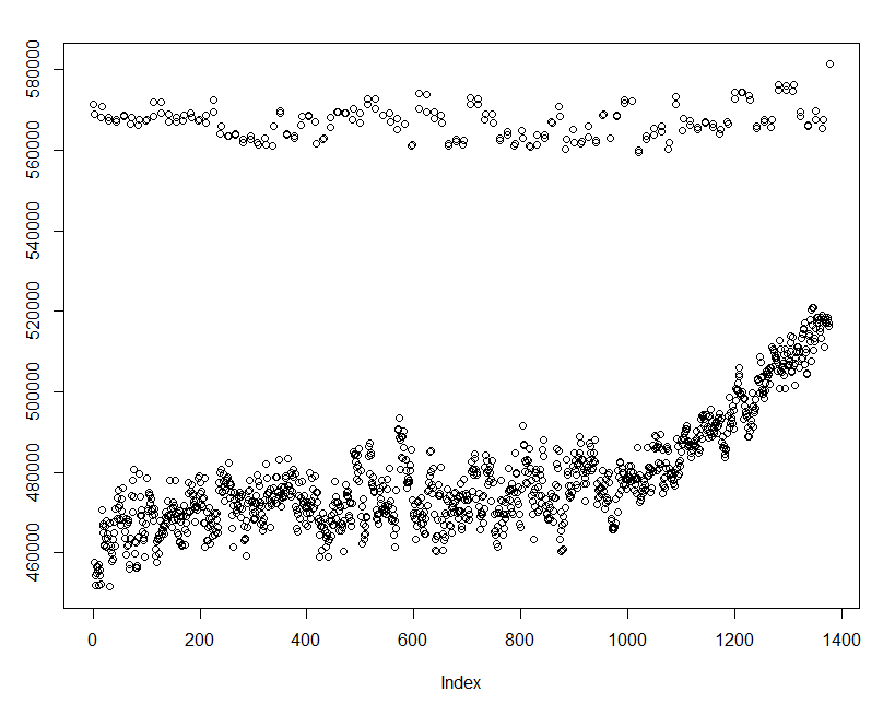
This is great! There’s a clear demarcation between the white separating lines and the strips.
## assume everything above 540,000 is a dividing line divides <- which(strips > 540000) divides <- divides[-1]divides <- rev(rev(divides)[-1])divides %<>% matrix(ncol = 2, byrow = TRUE)## split the original image into strips shredl <- apply(divides, 1, function(q) { shred[, (q[1]+1):(q[2]-1), ] })
Now we have a list of strips, we need a function to compare two strips, and another one to bind two given strips together.
## takes two strips and compares the right v left edgescompare_strips <- function(stripsl, x, y) {r <- stripsl[[x]][, ncol(stripsl[[x]]), 1] - stripsl[[y]][, 1, 1]g <- stripsl[[x]][, ncol(stripsl[[x]]), 2] - stripsl[[y]][, 1, 2]b <- stripsl[[x]][, ncol(stripsl[[x]]), 3] - stripsl[[y]][, 1, 3]r %<>% abs() %>% sum()g %<>% abs() %>% sum()b %<>% abs() %>% sum()r+g+b }## bind two given strips togetherbindem <- function(stripsl, lft, rgt) {bound <- abind(stripsl[[lft]], stripsl[[rgt]], along=2)#[,,1] %>% image()stripsl <- c(stripsl[-c(lft, rgt)], list(bound)) }
Now the hard work is done, we can run the strips through:
for (qq in 1:99) {wm <- sapply(2:length(shredl), function(q) compare_strips(shredl, 1, q)) %>% which.min() + 1shredl <- bindem(shredl, 1, wm)}
And finally, we’ll export the solution to see whether its legible.
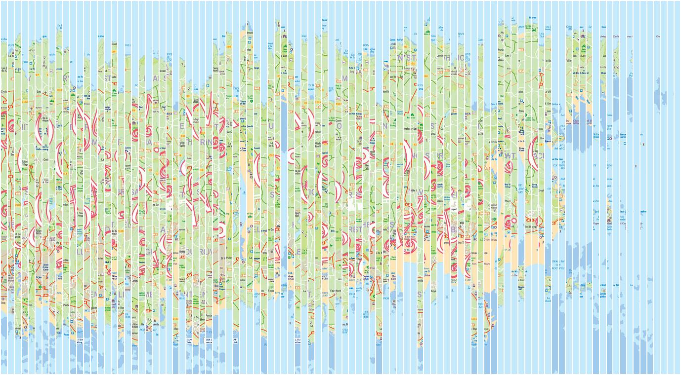
(shredl[[length(shredl)]]/255) %>%jpeg::writeJPEG(target = paste0(dr, "GC4F5HY_shredded-jps09_solved.jpg"))
And here it is. I’ve censored the final coordinates out of respect for the cache owner. You can see the algorithm for stitching together the strips hasn’t worked perfectly, but the map and coordinates are legible. Success!

And yes, the coordinates are upside down. That’s a feature of the puzzle, I guess. The strips I’ve output are oriented the same way as in the original, as you can see from the town names in the map itself.
GC6CQT9 Denken tut nicht weh / myślenie nie boli – 06

This puzzle cache is in Mecklenburg-Vorpommern, Germany. The description is in German and repeated in Polish. Annoyingly, the puzzle instructions are in an image, so you can’t copy and paste the text into translation software. I retyped the German text into Google Translate and got the gist of it.
You have a weighing scales and five different weights. In combination they can be used to measure the weight of any unknown object from 1kg to 121kg. All weights are whole numbers.
To illustrate, imagine you have amongst your five weights, a 12kg weight and a 4kg weight. Clearly, you could successfully weigh another object of 12kg or 4kg. Also, by placing them together you could weigh something 16kg, and by placing the 4kg on one side and the 12kg on the other, you could determine the weight of an 8kg object.
This is probably some old classic, but it looked like an interesting programming puzzle. I didn’t try to google it, but instead thought about how to limit the scope of my search.
Firstly, it’s not obvious that the heaviest weight must be less than 121kg. For example, you can make 115kg using 100+15, but equally 130-15. I decided arbitrarily that I would test combinations up to 150kg.
Secondly, the total weight of the five weights must be at least 121kg. Obviously it’s not possible to measure the weight of any object in excess what you have available to put against it.
The constraints were not yet enough to make this a tractable problem. Even taking into account four of the five weights, the number of combinations for different weights from 1-150kg is 486,246,600. Clearly, I needed a way to narrow the search.
Looking on the cache page, the formula for the location gave me a way in:N 53 52.(B-A)(E/C)(D/C+B) E 014 08.(C/B+A)({E-D}/C)(E/D)
(assuming A<B<C<D<E)
This is very helpful! The format of the coordinates means you cannot have fractions: we know that E/C is an integer, as is D/C, C/B, (E-D)/C and E/D. By now I was starting to suspect what the solution would be, but I followed it through programmatically.
I set up the 5 objects with the values 1:150 and then made a data frame using the crossing function (from the tidyr package):
library(tidyverse)
library(magrittr)
a <- b <- c <- d <- e <- 1:150
dafr <- crossing(b, c)
This contains all 22500 permutations of two of the weights. But we can filter these rows straight away, because C>A, and C/A is an integer:
dafr %<>%filter(c > b) %>%filter((c/b)%%1==0)
This reduces the combinations down to 630. A good start! Now we can add in another weight:
dafr %<>%crossing(e) %>%filter(e > c) %>%filter((e/c)%%1==0) %>%filter(e/c < 10)
Note that I’ve also filtered by E/C being less than ten.
In short, the whole of this step produces 252 combinations of weights
dafr %<>%crossing(e) %>%filter(e > c) %>%filter((e/c)%%1==0) %>%filter(e/c < 10) %>%filter((c/b)%%1==0) %>%crossing(a) %>%filter(b > a) %>%filter(b-a < 10) %>%filter(c/b+a < 10) %>%crossing(d) %>%filter(d > c) %>%filter(e > d) %>%filter((d/c)%%1==0) %>%filter((d/c)+b < 10) %>%filter(((e-d)/c)%%1==0) %>%filter(((e-d)/c) < 10) %>%filter((e/d)%%1==0) %>%filter((e/d) < 10) %>%select(a, b, c, d, e) %>%mutate(max=a+b+c+d+e) %>%filter(max > 120)
They are the weightsets that might work. But only one of those is the answer. So which one?
To answer that, we need to consider some way of finding all of the internal combinations of each of those weightsets. Consider the first line: 1 2 10 40 80. Obviously we can make 1kg, 2kg, 3kg (1+2), 7kg (10-2-1), and so on.
In order to make a combined weight, we can take each weight in turn and weight positively, negatively, or not use it. So the 7kg result above is -1*1 + -1*2 + 1*10 + 0*40 + 0*80.
I created new variables in the data frame, called v, w, x, y, and z. These held every permutation of -1, 0, and 1, using the crossing function:
v <- w <- x <- y <- z <- -1:1dafr %<>% crossing(v, w, x, y, z)
Then, multiplying the a-e by v-z, I had every possible use-combination of all the valid weightsets:
dafr %<>%mutate(av=av, bw=bw, cx=cx, dy=dy, ez=e*z) %>%mutate(weigh=av+bw+cx+dy+ez) %>%select(a, b, c, d, e, weigh)
Finally, I counted up how many separate weights could be achieved per weightset:
dafr %>%filter(weigh > 0) %>%filter(weigh < 122) %>%unique() %>%group_by(a, b, c, d, e) %>%summarise(n=n()) %>%arrange(-n)
As expected, there was one weightset at the top of that table that covered all 121 possibilities, meaning I just needed to plug the values into the formula by hand and the puzzle cache was solved.
I won’t show the answer here because most cache owners don’t appreciate their mysteries being spoiled by having the solution posted online. But the programmatic approach worked in this case, with a little thought to circumvent the obvious issues of naively working through hundreds of millions of combinations.
That’s not the say the programmatic approach is the best way to approach caches like this. Looking at the answer, an obvious heuristic approach to producing the answer reveals itself to me. And it was the way I “saw” half way through creating the programme. But sometimes the intelligent way is only obvious after the fact, and the programmatic approach can help you learn something about the nature of the problem.
